2023. 11. 12. 20:14ㆍ컴퓨터비전
Line Detector

Hozontal mask를 예를 들어보면
이 mask를 통과시킨다면 수직방향으로 값의 차이가 있으면 0이 아닌 값을 반환,
수직방향으로 값의 차이가 없다면 0인 값을 반환.
-> y방향으로의 변화량을 보기 위함.
다른 mask들도 같은 메커니즘이다.
mask의 있는 값들을 모두 더하면 0이 되어야 한다.
Edge detection
: 밝기가 급격히 변하는 부분을 발견하는 것
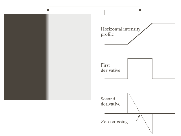
Zero crossing
: intensity를 2차 미분했을 때 최고점과 최저점을 직선으로 이었을 때
0이 되는 부분을 에지라고 정의하면 바람직하다.
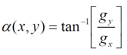
Gradient
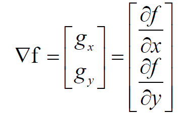


루트는 연산속도가 느려서 절댓값으로 근사해서 계산한다.
Effect of noise

작은 noise가 섞였을 뿐이지만 여러 번 미분할수록 티가 많이 난다.
Three Fundamental Steps
1. noise를 줄이기 위해 이미지 smoothing
2. edge point들 detection 하기
3. Edge localization
1. Smoothing
Gaussian Filter
- 가우시안 분포는 중심을 기준으로 대칭을 이룸
- 총면적은 1
- 중심에 더 많은 weight를 주고 거리가 멀어질수록 weight가 감소하는 kenel을 갖는다.
- 시그마값이 커질수록 weight는 고르게 한다
-> 노이즈가 많으면 시그마값을 크게 해야 한다, 강한 edge만 살린다.
시그마값이 작아질수록 중심에 더 큰 weight를 준다.
-> 노이즈가 적으면 시그마값을 작게 해야 한다, 약한 edge도 확인가


f는 noise가 섞인 이미지
g는 가우시안 필터
-> convolution 하면 noise가 제거

linear 하므로 g를 먼저 미분하고 f와 convolution해도
결과는 같아진다.
2. Edge points detection
sobel mask
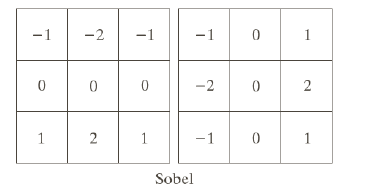
왼쪽이 y방향 edge 탐지, 오른쪽이 x방향 edge 탐지
-> x의 변화량으로는 y방향의 edge를 검출할 수 있으며,
y의 변화량으로는 x방향의 edge를 검출할 수 있다.
Thresholding
: 이미지에서 가장 높은 픽셀 값의 threshold=t%인 부분들만 선택
#include <opencv2/opencv.hpp>
#include <vector>
using namespace cv;
using namespace std;
Mat Filter(const Mat& img, const vector <vector <double> >& kernel,int ksize) {
int center = ksize / 2; //커널의 중심 인덱스
Mat result = Mat::zeros(img.rows, img.cols, img.type()); //zero padding
for (int y = center;y < img.rows - center;y++) {
for (int x = center;x < img.cols - center;x++) {
double sum = 0.0;
//convolution
for (int i = -center;i <= center;i++) {
for (int j = -center;j <= center;j++) {
sum += (img.at<uchar>(y + i, x + j) * kernel[i + center][j + center]);
}
}
result.at<uchar>(y, x) = saturate_cast<uchar>(sum); //0~255범위를 넘지 않게 하기 위해
}
}
return result;
}
Mat Threshold(const Mat& img, double threshold) {
Mat result = img.clone();
double pixel = 0;
for (int y = 0;y < img.rows;y++) {
for (int x = 0;x < img.cols;x++) {
pixel = img.at<uchar>(y, x);
if (pixel > threshold) {
result.at<uchar>(y, x) = img.at<uchar>(y, x);
}
else
result.at<uchar>(y, x) = 0;
}
}
return result;
}
Mat Sobel(const Mat& img) {
vector<vector <double> > sobel_x = {
{-1,0,1},
{-2,0,2},
{-1,0,1}
};
vector<vector <double> > sobel_y = {
{-1,-2,-1},
{0,0,0},
{1,2,1}
};
Mat gradient_x = Filter(img, sobel_x, 3); //x에 대하여 필터링
Mat grdient_y = Filter(img, sobel_y, 3); //y에 대하여 필터링
Mat result1, result2, result3;
convertScaleAbs(gradient_x, result1); // |gx|
convertScaleAbs(grdient_y, result2); //|gy|
add(result1, result2, result3, noArray(), img.type());
return result3;
}
Mat Sobel_x(const Mat& img) {
vector<vector <double> > sobel_x = {
{-1,0,1},
{-2,0,2},
{-1,0,1}
};
Mat gradient_x = Filter(img, sobel_x, 3); //x에 대하여 필터링
Mat result1;
convertScaleAbs(gradient_x, result1); // |gx|
return result1;
}
Mat Sobel_y(const Mat& img) {
vector<vector <double> > sobel_y = {
{-1,-2,-1},
{0,0,0},
{1,2,1}
};
Mat grdient_y = Filter(img, sobel_y, 3); //y에 대하여 필터링
Mat result1;
convertScaleAbs(grdient_y, result1); //|gy|
return result1;
}
int main() {
Mat img = imread("Lena512.jpg",IMREAD_GRAYSCALE);
Mat result1,result2;
result1 = Sobel_x(img);
imshow("sobel x", result1);
result1 = Sobel_y(img);
imshow("sobel y", result1);
result1 = Sobel(img);
imshow("sobel x+y", result1);
double t = 0; //threshold
t = 255 * 0.49;
result2 = Threshold(result1, t);
imshow("sobel,t=49%", result2);
Mat result3,result4,result5;
GaussianBlur(img, result3, Size(3,3), 0);
result3 = Sobel(result3);
result3 = Threshold(result3, t);
imshow("Gaussian+Sobel", result3);
GaussianBlur(img, result5, Size(7,7), 0);
result5 = Sobel(result5);
result5 = Threshold(result5, t);
imshow("Gaussian+Sobel7*7", result5);
//커널의 크기가 클수록 노이즈가 더욱 제거됨
waitKey(0);
return 0;
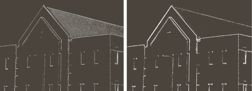
}Canny Edge Detector
3가지 기본 목표
- 낮은 오차율
- edge point들이 잘 localized 돼야 함
-> 어디가 edge인지 정확히 구별해야 함
Hysteresis thresholding
: weak edge를 살릴지 말지 주변을 보고 결정하는 방법
- threshold 2개를 정의한다: Low and High
- Low보다 작다면 edge가 아니다
- High보다 크다면 strong edge이다
- Low와 High 사이라면 weak edge이다

3. edge가 하나만 존재하면 하나로 표현
(여러 개로 표시하지 않고)
Non-maximum suppression
: 두꺼운 선은 어떻게 표현할 것인가에 해결법
(single edge point를 얻기 위한 기법)
-> 최댓값만 선택한다

Hough transform
: line detecting 기술
방법
: 가능한 모든 라인에 대해 투표를 진행해 기록하고
가장 많은 표를 받은 라인을 선택한다.

그림과 같이 변형하면 직선이 점 하나로 표현이 가능해진다.
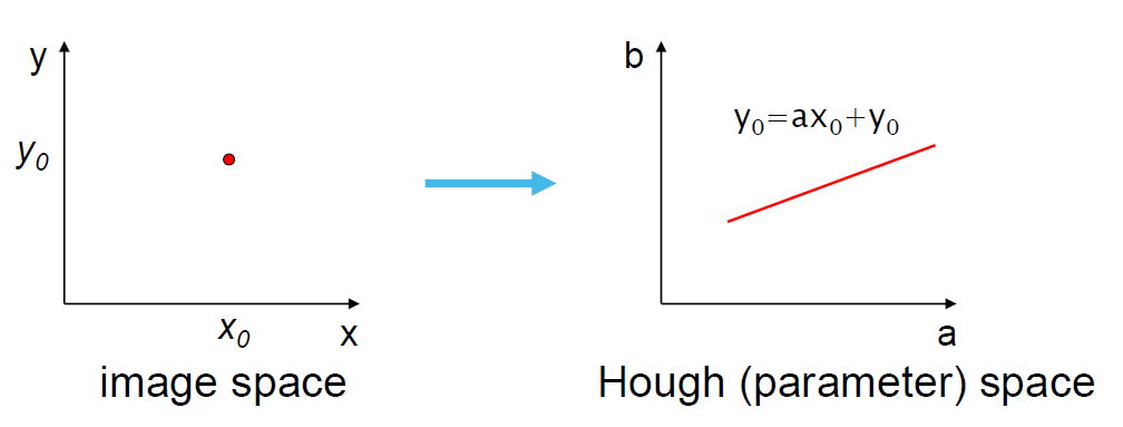
점을 직선으로 표현하는 것 또한 가능.

Hough space에서 교점을 찾기
-> 교점이 생긴다는 건 원래 영상을 이으면 직선이 된다는 뜻
'컴퓨터비전' 카테고리의 다른 글
| 과제하며 배운 opencv 함수 및 여러 정보 (2) | 2023.11.20 |
|---|---|
| Feature Detection and Matching (0) | 2023.11.14 |
| Image Restoration and Reconstruction (0) | 2023.11.10 |
| (opencv) visual studio에 적용하기 (0) | 2023.11.01 |
| Filtering in the Frequency Domain (1) | 2023.10.18 |